
Over a year ago (January 2025), I began development of my NHL data analysis library in Python. The main component of the library, the play-by-play scraper, was the first feature I finished and utilized to begin my own amateur hockey analytics work. After obtaining play-by-play data from the variety of data the NHL provides on a game-by-game basis (such as API endpoints and HTML reports) from the 2010-2011 season to the recently completed 2025-2026 regular season, I now possess a wealth of official NHL data.
Naturally, the next step was to begin work on developing the macrostats I plan to promote and provide to the public in the future. After developing an expected goals model, I began development of a set of similar models to serve as the base for my online player evaluations. My expected goals model is too similar to other public models to warrant its own article, at least for the time being.
As for the set of models, I elected to build models also similar to those already popular with the public. I, like many others, use regularized (L2 or Ridge) regression techniques; these are linear regression techniques that implement a penalty onto a given model’s predictors to force its coefficients closer to zero (at the generally slight cost of model fit). Models built in this way have become considerably popular in public sports analytics (particularly in basketball and hockey) as a way of estimating the influence of factors contributing to game outcomes, which cannot be strictly separated otherwise, and distributing credit amongst the individuals involved in game outcomes. Using the acquired NHL play-by-play data (filtering to regular-season only), I use two main data structures on which these models are trained: shift-by-shift and shot-by-shot models.
The shift-by-shift data structure condenses a stint of time in which all on-ice individuals (the skaters and goaltenders) remain the same. Shift changes integrated into the play-by-play data directly mark when a new stint should occur. Each row represents the offense team’s stint, with the on-ice NHL player IDs and coach names for the offensive and defensive teams marked alongside certain contextual terms. For each of these terms, a separate column is created in the dataset (as a predictor in the model), with one of the levels selected as the “reference level”. The reference level of a predictor is selected to compare each of the other terms’ levels against.
Three different models are developed with this data structure: even-strength shot rates, special-teams shot rates, and all strengths penalty rates. In the even-strength model, both teams are assigned offense rows in a single shift. For the special-team model, only the team on the power play is given an offensive row per shift. The all-strengths penalty model sets both teams to an offensive row per shift regardless of the strength state.
Once these terms are prepared, the target variables are included in the dataset. The target variable is what the team assigned as the offensive team for that shift. I have decided to encode the location of the target event per shift into a 100 by 85 (half-rink) grid, much like what was first accomplished by Micah Blake McCurdy (although encoding by one of 8500 coordinate locations instead of using a less coarse hex grid). The observed grid is then divided by the shift length (in seconds) and multiplied by 3600, transforming the values in the grid to a per-hour format by rink location. This ensures that our final estimates are individual impacts on the target variable per hour per (x, y) coordinate in the offensive half of the ice.
A separate model is ran for each target variable in each individual season in which play-by-play data can be converted to this shift-by-shift structure.
Each of the features in the model is displayed below:
-
Shot Rate Models: Fenwick, Corsi, shots, expected goals, and goals
-
Penalty Rate Model: penalty minutes
And for the model’s predictors (with their respective reference level):
-
Period Number: 1st period
-
Specific Strength State: 5v5 (even-strength and all-strengths models), 5v4 (special-teams model)
-
Score State (binning states in which a team is up or down three or more goals): Tied
-
Power-play and penalty-kill expiry states (even-strength model only): The reference level is a standard even-strength shift occurring after another even-strength shift
-
Team venue identifier: Away Team
-
Shift start location: On-the-fly
-
On-ice skaters; formatted such as “offense_8479987_20252026_BOS (Morgan Geekie in the 2025-2026 season for the Boston Bruins on the offensive side of the puck): League-average skater
-
Coaches (systems); formatted such as “defense_JON_COOPER_20252026_TBL (Jon Cooper coaching the 2025-2026 Tampa Bay Lightning on the defensive side of the puck); League-average coach
-
Coaches (score state); formatted such as “defense_lead_1_JON_COOPER_20252026_TBL (Jon Cooper coaching the 2025-2026 Tampa Bay Lightning on the defensive side of the puck when leading by a goal); League-average coach at that strength state (seven score states, both on offense and defense)
Individual and contextual estimations (coefficients of the model predictors) of impact on the target variable in that season are obtained after the model is fitted, using penalties selected based on prior work (rather than derived per model due to computational restraints). Coefficients are encoded into the aforementioned 100 by 85 grid; 8500 coefficients are summed to obtain the total coefficients in the model.
The coefficients of a linear regression are the estimates of that predictor’s impact on the target variable when all other predictors are controlled for (set to zero). The penalty ensures the sum of the terms for each contextual and individual term is zero. The model intercept (when all of the predictors are zero) is interpreted as the reference-level impact on the target variable.
For example, if the intercept to the even-strength Fenwick model is 37, this is interpreted to mean that the estimated Fenwick shots generated per hour would be 37 when:
-
All on-ice skaters, coaching systems, and tied score state coaching impacts are league-average
-
The away team is on offense, the home team is on defense
-
Strength-state is at 5v5
-
The game is in the first period
-
The shift started in the neutral zone
-
The game is tied
-
The shift is preceded by another even-strength shift
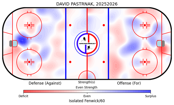
An individual’s coefficients are interpreted as their “isolated” impact on the target variable, both on offense (for) and defense (against). Defense grids are flipped (meaning that the range of x is from -100 to -1 rather than 0 to 99) to reflect the individual’s isolated impact on the target variable in their defensive zone.
Using the encoded grids in this way allows us, with some smoothing, to convert the coordinate impacts into a heatmap, which provides additional information on individual influences on shot rates. An example is provided below:
[
](https://substackcdn.com/image/fetch/$s_!BWZw!,f_auto,q_auto:good,fl_progressive:steep/https%3A%2F%2Fsubstack-post-media.s3.amazonaws.com%2Fpublic%2Fimages%2F1a710657-f2e5-4472-a3f7-bb8e47ba4e27_680x412.png)
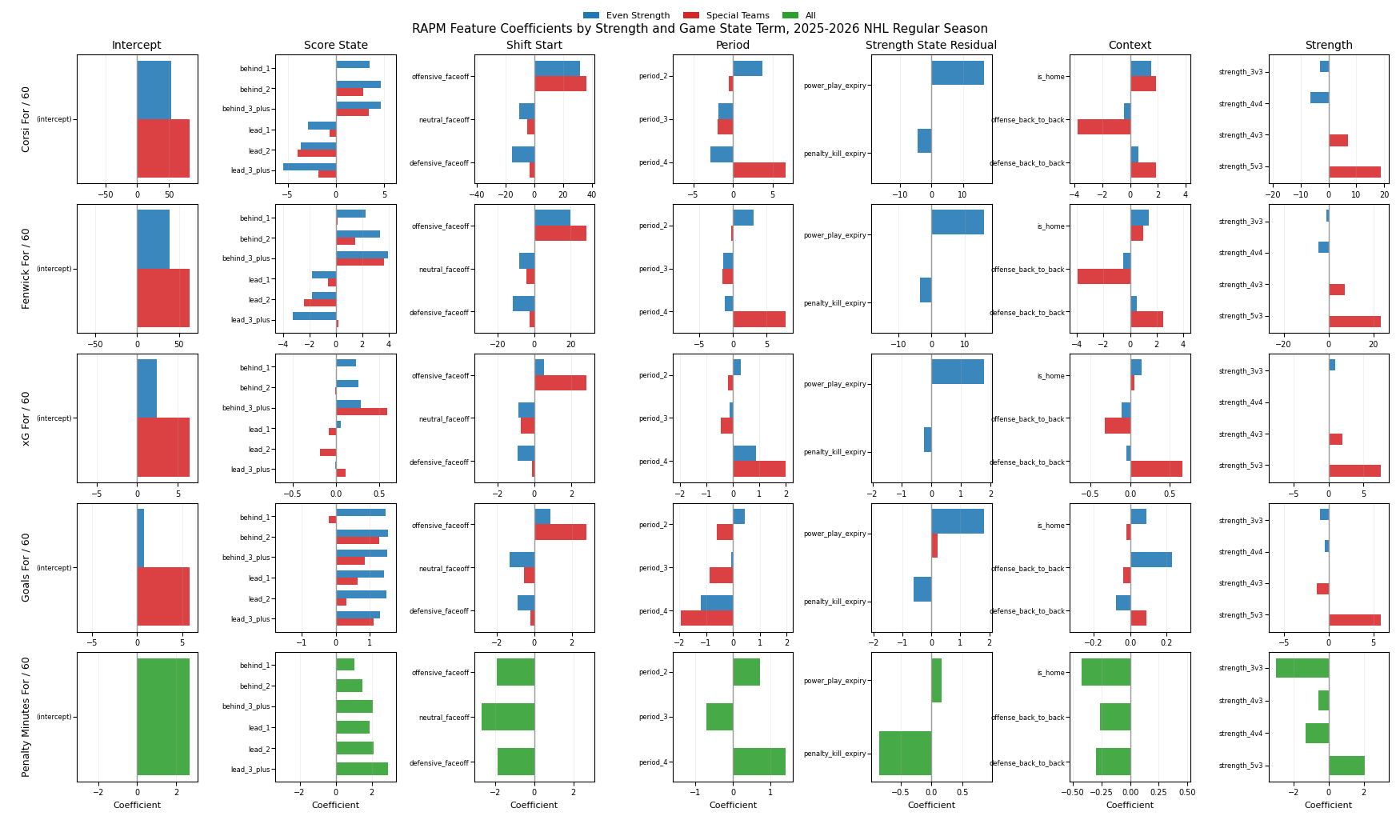
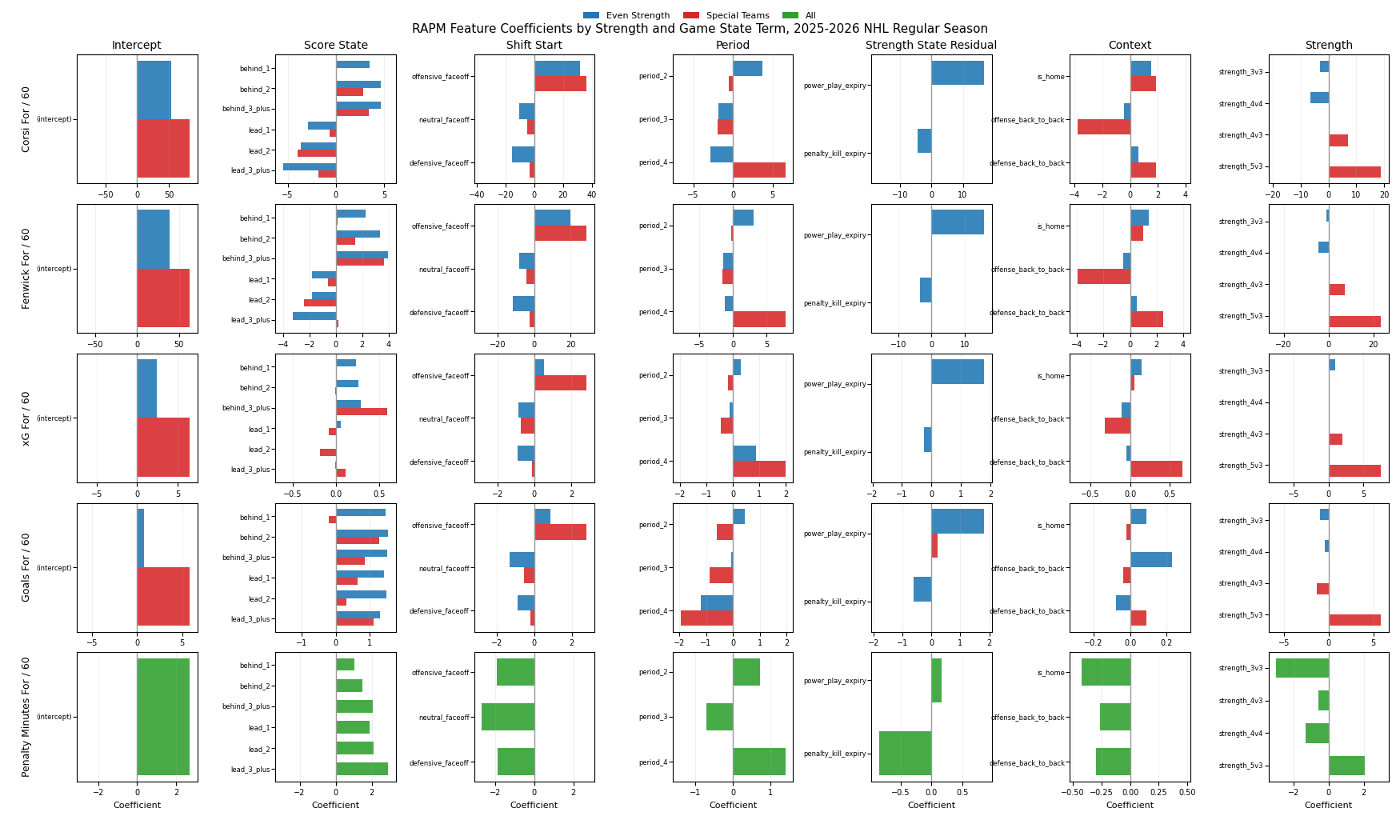
The summed contextual terms for the 2025-2026 season are provided here:
[
](https://substackcdn.com/image/fetch/$s_!m-SF!,f_auto,q_auto:good,fl_progressive:steep/https%3A%2F%2Fsubstack-post-media.s3.amazonaws.com%2Fpublic%2Fimages%2F74f1687b-77e3-4b4c-aef5-cfaa10a92e5e_1750x1050.png)
The other data, structured from the obtained play-by-play data, is far simpler. The data is filtered down to Fenwick events only (missed shots, shots on goal, and goals). The IDs for the shooter, on-ice skaters for the shooting team, and the goaltender facing the shot are encoded the same way as in the shift-by-shift data. Instead of marking each of the on-ice players for the shooting team with a binary value (on the ice or not), the probability that they contributed a primary or secondary shot assist is utilized (based on positional probabilities derived from manually tracked data in the AllThreeZones project). For goals, these are tracked by the NHL, so the shot assist probabilities for these events are binary values only.
Next, a regularized logistic regression is fit to this data, using the shot’s flag (if it was a goal or not) as the target variable and the expected goals of the shot (which is implied to be taken by a league-average shooter and faced by a league-average goaltender in the model) as a predictor, alongside the shooter, goalie, and passer terms described above. The expected goals encode all the contextual features used to estimate the probability of that shot converting, including the distance of the shot from the goal, the time in the game, the time from the last event, and more.
Our resulting coefficients are the estimated change in probability of a goal occurring provided by that predictor, with all other predictors set to zero. After these coefficients are obtained, I convert them to a “per-shot” impact on goal-conversion using the average slope of the logistic curve in the data and multiplying them by the model’s predictions. These scaled estimates can be used to approximate an above-expected (above-average) value for each player in a shooter, passing, or goaltending context when accounting for the quality of the other two contexts.
With these models completed, I can now continue my own path forward to embed the sport’s understanding into analyzing prior and current league results, as well as simulating and predicting future results. I plan to update this write-up in the near future, either when the models are modified in any way or when technical or ambiguous aspects of the models described are addressed further, if (or when) requested by readers.
Lots of prior work (especially that by EvolvingHockey, HockeyStats.com, and Micah Blake McCurdy at HockeyViz.com) not only inspired the work described here but also, to some degree, contributed to it by providing their process for obtaining models of their own. Developing each of these models provides me with experience with the technical skills required to progress in data science, in addition to acquiring independence in achieving a higher level of analysis of a sport that I deeply enjoy following.